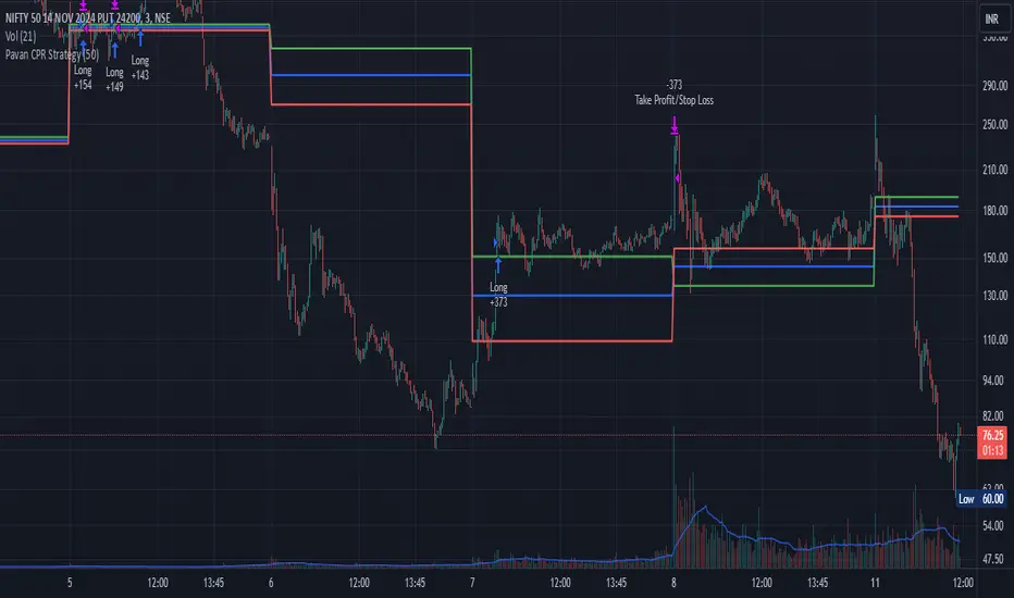
Pavan CPR Strategy Pavan CPR Strategy (Pine Script)
The Pavan CPR Strategy is a trading system based on the Central Pivot Range (CPR), designed to identify price breakouts and generate long trade signals. This strategy uses key CPR levels (Pivot, Top CPR, and Bottom CPR) calculated from the daily high, low, and close to inform trade decisions. Here's an overview of how the strategy works:
Key Components:
CPR Calculation:
The strategy calculates three critical CPR levels for each trading day:
Pivot (P): The central value, calculated as the average of the high, low, and close prices.
Top Central Pivot (TC): The midpoint of the daily high and low, acting as the resistance level.
Bottom Central Pivot (BC): Derived from the pivot and the top CPR, providing a support level.
The script uses request.security to fetch these CPR values from the daily timeframe, even when applied on intraday charts.
Trade Entry Condition:
A long position is initiated when:
The current price crosses above the Top CPR level (TC).
The previous close was below the Top CPR level, signaling a breakout above a key resistance level.
This condition aims to capture upward momentum as the price breaks above a significant level.
Exit Strategy:
Take Profit: The position is closed with a profit target set 50 points above the entry price.
Stop Loss: A stop loss is placed at the Pivot level to protect against unfavorable price movements.
Visual Reference:
The script plots the three CPR levels on the chart:
Pivot: Blue line.
Top CPR (TC): Green line.
Bottom CPR (BC): Red line.
These plotted levels provide visual guidance for identifying potential support and resistance zones.
Use Case:
The Pavan CPR Strategy is ideal for intraday traders who want to capitalize on price movements and breakouts above critical CPR levels. It provides clear entry and exit signals based on price action and is best used in conjunction with proper risk management.
Note: The strategy is written in Pine Script v5 for use on TradingView, and it is recommended to backtest and optimize it for the asset or market you are trading.
在腳本中搜尋"the strat"
FTMO Rules MonitorFTMO Rules Monitor: Stay on Track with Your FTMO Challenge Goals
TLDR; You can test with this template whether your strategy for one asset would pass the FTMO challenges step 1 then step 2, then with real money conditions.
Passing a prop firm challenge is ... challenging.
I believe a toolkit allowing to test in minutes whether a strategy would have passed a prop firm challenge in the past could be very powerful.
The FTMO Rules Monitor is designed to help you stay within FTMO’s strict risk management guidelines directly on your chart. Whether you’re aiming for the $10,000 or the $200,000 account challenge, this tool provides real-time tracking of your performance against FTMO’s rules to ensure you don’t accidentally breach any limits.
NOTES
The connected indicator for this post doesn't matter.
It's just a dummy double supertrends (see below)
The strategy results for this script post does not matter as I'm posting a FTMO rules template on which you can connect any indicator/strategy.
//@version=5
indicator("Supertrends", overlay=true)
// Supertrend 1 Parameters
var string ST1 = "Supertrend 1 Settings"
st1_atrPeriod = input.int(10, "ATR Period", minval=1, maxval=50, group=ST1)
st1_factor = input.float(2, "Factor", minval=0.5, maxval=10, step=0.5, group=ST1)
// Supertrend 2 Parameters
var string ST2 = "Supertrend 2 Settings"
st2_atrPeriod = input.int(14, "ATR Period", minval=1, maxval=50, group=ST2)
st2_factor = input.float(3, "Factor", minval=0.5, maxval=10, step=0.5, group=ST2)
// Calculate Supertrends
= ta.supertrend(st1_factor, st1_atrPeriod)
= ta.supertrend(st2_factor, st2_atrPeriod)
// Entry conditions
longCondition = direction1 == -1 and direction2 == -1 and direction1 == 1
shortCondition = direction1 == 1 and direction2 == 1 and direction1 == -1
// Optional: Plot Supertrends
plot(supertrend1, "Supertrend 1", color = direction1 == -1 ? color.green : color.red, linewidth=3)
plot(supertrend2, "Supertrend 2", color = direction2 == -1 ? color.lime : color.maroon, linewidth=3)
plotshape(series=longCondition, location=location.belowbar, color=color.green, style=shape.triangleup, title="Long")
plotshape(series=shortCondition, location=location.abovebar, color=color.red, style=shape.triangledown, title="Short")
signal = longCondition ? 1 : shortCondition ? -1 : na
plot(signal, "Signal", display = display.data_window)
To connect your indicator to this FTMO rules monitor template, please update it as follow
Create a signal variable to store 1 for the long/buy signal or -1 for the short/sell signal
Plot it in the display.data_window panel so that it doesn't clutter your chart
signal = longCondition ? 1 : shortCondition ? -1 : na
plot(signal, "Signal", display = display.data_window)
In the FTMO Rules Monitor template, I'm capturing this external signal with this input.source variable
entry_connector = input.source(close, "Entry Connector", group="Entry Connector")
longCondition = entry_connector == 1
shortCondition = entry_connector == -1
🔶 USAGE
This indicator displays essential FTMO Challenge rules and tracks your progress toward meeting each one. Here’s what’s monitored:
Max Daily Loss
• 10k Account: $500
• 25k Account: $1,250
• 50k Account: $2,500
• 100k Account: $5,000
• 200k Account: $10,000
Max Total Loss
• 10k Account: $1,000
• 25k Account: $2,500
• 50k Account: $5,000
• 100k Account: $10,000
• 200k Account: $20,000
Profit Target
• 10k Account: $1,000
• 25k Account: $2,500
• 50k Account: $5,000
• 100k Account: $10,000
• 200k Account: $20,000
Minimum Trading Days: 4 consecutive days for all account sizes
🔹 Key Features
1. Real-Time Compliance Check
The FTMO Rules Monitor keeps track of your daily and total losses, profit targets, and trading days. Each metric updates in real-time, giving you peace of mind that you’re within FTMO’s rules.
2. Color-Coded Visual Feedback
Each rule’s status is shown clearly with a ✓ for compliance or ✗ if the limit is breached. When a rule is broken, the indicator highlights it in red, so there’s no confusion.
3. Completion Notification
Once all FTMO requirements are met, the indicator closes all open positions and displays a celebratory message on your chart, letting you know you’ve successfully completed the challenge.
4. Easy-to-Read Table
A table on your chart provides an overview of each rule, your target, current performance, and whether you’re meeting each goal. The table adjusts its color scheme based on your chart settings for optimal visibility.
5. Dynamic Position Sizing
Integrated ATR-based position sizing helps you manage risk and avoid large drawdowns, ensuring each trade aligns with FTMO’s risk management principles.
Daveatt

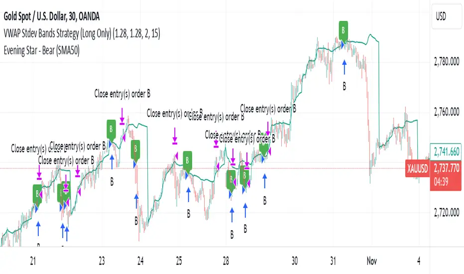
VWAP Stdev Bands Strategy (Long Only)The VWAP Stdev Bands Strategy (Long Only) is designed to identify potential long entry points in trending markets by utilizing the Volume Weighted Average Price (VWAP) and standard deviation bands. This strategy focuses on capturing upward price movements, leveraging statistical measures to determine optimal buy conditions.
Key Features:
VWAP Calculation: The strategy calculates the VWAP, which represents the average price a security has traded at throughout the day, weighted by volume. This is an essential indicator for determining the overall market trend.
Standard Deviation Bands: Two bands are created above and below the VWAP, calculated using specified standard deviations. These bands act as dynamic support and resistance levels, providing insight into price volatility and potential reversal points.
Trading Logic:
Long Entry Condition: A long position is triggered when the price crosses below the lower standard deviation band and then closes above it, signaling a potential price reversal to the upside.
Profit Target: The strategy allows users to set a predefined profit target, closing the long position once the specified target is reached.
Time Gap Between Orders: A customizable time gap can be specified to prevent multiple orders from being placed in quick succession, allowing for a more controlled trading approach.
Visualization: The VWAP and standard deviation bands are plotted on the chart with distinct colors, enabling traders to visually assess market conditions. The strategy also provides optional plotting of the previous day's VWAP for added context.
Use Cases:
Ideal for traders looking to engage in long-only positions within trending markets.
Suitable for intraday trading strategies or longer-term approaches based on market volatility.
Customization Options:
Users can adjust the standard deviation values, profit target, and time gap to tailor the strategy to their specific trading style and market conditions.
Note: As with any trading strategy, it is important to conduct thorough backtesting and analysis before live trading. Market conditions can change, and past performance does not guarantee future results.
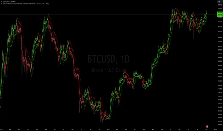
RBF Kijun Trend System [InvestorUnknown]The RBF Kijun Trend System utilizes advanced mathematical techniques, including the Radial Basis Function (RBF) kernel and Kijun-Sen calculations, to provide traders with a smoother trend-following experience and reduce the impact of noise in price data. This indicator also incorporates ATR to dynamically adjust smoothing and further minimize false signals.
Radial Basis Function (RBF) Kernel Smoothing
The RBF kernel is a mathematical method used to smooth the price series. By calculating weights based on the distance between data points, the RBF kernel ensures smoother transitions and a more refined representation of the price trend.
The RBF Kernel Weighted Moving Average is computed using the formula:
f_rbf_kernel(x, xi, sigma) =>
math.exp(-(math.pow(x - xi, 2)) / (2 * math.pow(sigma, 2)))
The smoothed price is then calculated as a weighted sum of past prices, using the RBF kernel weights:
f_rbf_weighted_average(src, kernel_len, sigma) =>
float total_weight = 0.0
float weighted_sum = 0.0
// Compute weights and sum for the weighted average
for i = 0 to kernel_len - 1
weight = f_rbf_kernel(kernel_len - 1, i, sigma)
total_weight := total_weight + weight
weighted_sum := weighted_sum + (src * weight)
// Check to avoid division by zero
total_weight != 0 ? weighted_sum / total_weight : na
Kijun-Sen Calculation
The Kijun-Sen, a component of Ichimoku analysis, is used here to further establish trends. The Kijun-Sen is computed as the average of the highest high and the lowest low over a specified period (default: 14 periods).
This Kijun-Sen calculation is based on the RBF-smoothed price to ensure smoother and more accurate trend detection.
f_kijun_sen(len, source) =>
math.avg(ta.lowest(source, len), ta.highest(source, len))
ATR-Adjusted RBF and Kijun-Sen
To mitigate false signals caused by price volatility, the indicator features ATR-adjusted versions of both the RBF smoothed price and Kijun-Sen.
The ATR multiplier is used to create upper and lower bounds around these lines, providing dynamic thresholds that account for market volatility.
Neutral State and Trend Continuation
This indicator can interpret a neutral state, where the signal is neither bullish nor bearish. By default, the indicator is set to interpret a neutral state as a continuation of the previous trend, though this can be adjusted to treat it as a truly neutral state.
Users can configure this setting using the signal_str input:
simple string signal_str = input.string("Continuation of Previous Trend", "Treat 0 State As", options = , group = G1)
Visual difference between "Neutral" (Bottom) and "Continuation of Previous Trend" (Top). Click on the picture to see it in full size.
Customizable Inputs and Settings:
Source Selection: Choose the input source for calculations (open, high, low, close, etc.).
Kernel Length and Sigma: Adjust the RBF kernel parameters to change the smoothing effect.
Kijun Length: Customize the lookback period for Kijun-Sen.
ATR Length and Multiplier: Modify these settings to adapt to market volatility.
Backtesting and Performance Metrics
The indicator includes a Backtest Mode, allowing users to evaluate the performance of the strategy using historical data. In Backtest Mode, a performance metrics table is generated, comparing the strategy's results to a simple buy-and-hold approach. Key metrics include mean returns, standard deviation, Sharpe ratio, and more.
Equity Calculation: The indicator calculates equity performance based on signals, comparing it against the buy-and-hold strategy.
Performance Metrics Table: Detailed performance analysis, including probabilities of positive, neutral, and negative returns.
Alerts
To keep traders informed, the indicator supports alerts for significant trend shifts:
// - - - - - ALERTS - - - - - //{
alert_source = sig
bool long_alert = ta.crossover (intrabar ? alert_source : alert_source , 0)
bool short_alert = ta.crossunder(intrabar ? alert_source : alert_source , 0)
alertcondition(long_alert, "LONG (RBF Kijun Trend System)", "RBF Kijun Trend System flipped ⬆LONG⬆")
alertcondition(short_alert, "SHORT (RBF Kijun Trend System)", "RBF Kijun Trend System flipped ⬇Short⬇")
//}
Important Notes
Calibration Needed: The default settings provided are not optimized and are intended for demonstration purposes only. Traders should adjust parameters to fit their trading style and market conditions.
Neutral State Interpretation: Users should carefully choose whether to treat the neutral state as a continuation or a separate signal.
Backtest Results: Historical performance is not indicative of future results. Market conditions change, and past trends may not recur.
Dual Momentum StrategyThis Pine Script™ strategy implements the "Dual Momentum" approach developed by Gary Antonacci, as presented in his book Dual Momentum Investing: An Innovative Strategy for Higher Returns with Lower Risk (McGraw Hill Professional, 2014). Dual momentum investing combines relative momentum and absolute momentum to maximize returns while minimizing risk. Relative momentum involves selecting the asset with the highest recent performance between two options (a risky asset and a safe asset), while absolute momentum considers whether the chosen asset has a positive return over a specified lookback period.
In this strategy:
Risky Asset (SPY): Represents a stock index fund, typically more volatile but with higher potential returns.
Safe Asset (TLT): Represents a bond index fund, which generally has lower volatility and acts as a hedge during market downturns.
Monthly Momentum Calculation: The momentum for each asset is calculated based on its price change over the last 12 months. Only assets with a positive momentum (absolute momentum) are considered for investment.
Decision Rules:
Invest in the risky asset if its momentum is positive and greater than that of the safe asset.
If the risky asset’s momentum is negative or lower than the safe asset's, the strategy shifts the allocation to the safe asset.
Scientific Reference
Antonacci's work on dual momentum investing has shown the strategy's ability to outperform traditional buy-and-hold methods while reducing downside risk. This approach has been reviewed and discussed in both academic and investment publications, highlighting its strong risk-adjusted returns (Antonacci, 2014).
Reference: Antonacci, G. (2014). Dual Momentum Investing: An Innovative Strategy for Higher Returns with Lower Risk. McGraw Hill Professional.

HBK Price Action Strategy HBKPrice Action Strategy for XAUUSD with a Favorable Risk-Reward Ratio
Understanding the Strategy:
This strategy leverages price action principles to identify potential entry and exit points for XAUUSD on a 5-minute timeframe. The core idea is to identify price action patterns that suggest a high probability of a particular direction, and then to set stop-loss and take-profit levels to manage risk and reward.
Key Price Action Patterns to Watch:
Pin Bar: A pin bar is a candlestick with a long wick in one direction and a small body in the opposite direction. It often signals a reversal in the current trend.
Inside Bar: An inside bar forms when the current candle's high is lower than the previous candle's high, and the current candle's low is higher than the previous candle's low. It often indicates indecision or a potential breakout.
Engulfing Pattern: An engulfing pattern occurs when the current candle completely engulfs the previous candle. A bullish engulfing pattern signals a potential uptrend, while a bearish engulfing pattern signals a potential downtrend.
Risk-Reward Ratio:
A favorable risk-reward ratio is crucial for long-term trading success. Aim for a minimum risk-reward ratio of 1:2, meaning you risk $1 to potentially gain $2.
Entry and Exit Signals:
Long Entry:
Identify a bullish pin bar or engulfing pattern.
Wait for a confirmation candle to close above the pin bar's high or the engulfing pattern's high.
Place a stop-loss below the recent swing low.
Set a take-profit target at a key resistance level or a multiple of the stop-loss distance.
Short Entry:
Identify a bearish pin bar or engulfing pattern.
Wait for a confirmation candle to close below the pin bar's low or the engulfing pattern's low.
Place a stop-loss above the recent swing high.
Set a take-profit target at a key support level or a multiple of the stop-loss distance.
Additional Tips:
Use Support and Resistance Levels: Identify key support and resistance levels to set your stop-loss and take-profit targets.
Consider Market Sentiment: Pay attention to market sentiment and news events that may impact gold prices.
Manage Risk: Always use stop-loss orders to limit potential losses.
Be Patient: Don't force trades. Wait for high-probability setups.
Practice Discipline: Stick to your trading plan and avoid impulsive decisions.
Remember:
Price action trading requires practice and patience.
Backtest your strategy on historical data to refine your approach.
Always adapt to changing market conditions.
By following these guidelines and practicing disciplined risk management, you can increase your chances of success in trading XAUUSD on a 5-minute timeframe.

Multi Fibonacci Supertrend with Signals【FIbonacciFlux】Multi Fibonacci Supertrend with Signals (MFSS)
Overview
The Multi Fibonacci Supertrend with Signals (MFSS) is an advanced technical analysis tool that combines multiple Supertrend indicators using Fibonacci ratios to identify trend directions and potential trading opportunities.
Key Features
1. Fibonacci-Based Supertrend Levels
* Factor 1 (Weak) : 0.618 - The golden ratio
* Factor 2 (Medium) : 1.618 - The Fibonacci ratio
* Factor 3 (Strong) : 2.618 - The extension ratio
2. Visual Components
* Multi-layered Trend Lines
* Different line weights for easy identification
* Progressive transparency from Factor 1 to Factor 3
* Color-coded trend directions (Green for bullish, Red for bearish)
* Dynamic Fill Areas
* Gradient fills between price and trend lines
* Visual representation of trend strength
* Automatic color adjustment based on trend direction
* Signal Indicators
* Clear BUY/SELL labels on chart
* Position-adaptive signal placement
* High-visibility color scheme
3. Signal Generation Logic
The system generates signals based on two key conditions:
* Primary Condition :
* BUY : Price crossunder Supertrend2 (Factor 1.618)
* SELL : Price crossover Supertrend2 (Factor 1.618)
* Confirmation Filter :
* Signals only trigger when Supertrend3 confirms the trend direction
* Reduces false signals in volatile markets
Technical Details
Input Parameters
* ATR Period : 10 (default)
* Customizable for different market conditions
* Affects sensitivity of all Supertrend levels
* Factor Settings :
* All factors are customizable
* Default values based on Fibonacci sequence
* Minimum value: 0.01
* Step size: 0.01
Alert System
* Built-in alert conditions
* Customizable alert messages
* Real-time notification support
Use Cases
* Trend Trading
* Identify strong trend directions
* Filter out weak signals
* Confirm trend continuations
* Risk Management
* Multiple trend levels for stop-loss placement
* Clear entry and exit signals
* Trend strength visualization
* Market Analysis
* Multi-timeframe analysis capability
* Trend strength assessment
* Market structure identification
Benefits
* Reliability
* Based on proven Supertrend algorithm
* Enhanced with Fibonacci mathematics
* Multiple confirmation levels
* Clarity
* Clear visual signals
* Easy-to-interpret interface
* Reduced noise in signal generation
* Flexibility
* Customizable parameters
* Adaptable to different markets
* Suitable for various trading styles
Performance Considerations
* Optimized code structure
* Efficient calculation methods
* Minimal resource usage
Installation and Usage
Setup
* Add indicator to chart
* Adjust parameters if needed
* Enable alerts as required
Best Practices
* Use with other confirmation tools
* Adjust factors based on market volatility
* Consider timeframe appropriateness
Backtesting Results and Strategy Performance
This indicator is specifically designed for pullback trading with optimized risk-reward ratios in trend-following strategies. Below are the detailed backtesting results from our proprietary strategy implementation:
BTCUSDT Performance (Binance)
* Test Period: Approximately 7 years
* Risk-Reward Ratio: 2:1
* Take Profit: 8%
* Stop Loss: 4%
Key Metrics (BTCUSDT):
* Net Profit: +2,579%
* Total Trades: 551
* Win Rate: 44.8%
* Profit Factor: 1.278
* Maximum Drawdown: 42.86%
ETHUSD Performance (Binance)
* Risk-Reward Ratio: 4.33:1
* Take Profit: 13%
* Stop Loss: 3%
Key Metrics (ETHUSD):
* Net Profit: +8,563%
* Total Trades: 581
* Win Rate: 32%
* Profit Factor: 1.32
* Maximum Drawdown: 55%
Strategy Highlights:
* Optimized for pullback trading in strong trends
* Focus on high risk-reward ratios
* Proven effectiveness in major cryptocurrency pairs
* Consistent performance across different market conditions
* Robust profit factor despite moderate win rates
Note: These results are from our proprietary strategy implementation and should be used as reference only. Individual results may vary based on market conditions and implementation.
Important Considerations:
* The strategy demonstrates strong profitability despite lower win rates, emphasizing the importance of proper risk-reward ratios
* Higher drawdowns are compensated by significant overall returns
* The system shows adaptability across different cryptocurrencies with consistent profit factors
* Results suggest optimal performance in volatile crypto markets
Real Trading Examples
BTCUSDT 4-Hour Chart Analysis
Example of pullback strategy implementation on Bitcoin, showing clear trend definition and entry points
ETHUSDT 4-Hour Chart Analysis
Ethereum chart demonstrating effective signal generation during strong trends
BTCUSDT Detailed Signal Example (15-Minute Scalping)
Close-up view of signal generation and trend confirmation process on 15-minute timeframe, demonstrating the indicator's effectiveness for scalping operations
Chart Analysis Notes:
* Green and red zones clearly indicate trend direction
* Multiple timeframe confirmation visible through different Supertrend levels
* Clear entry signals during pullbacks in established trends
* Precise stop-loss placement opportunities below support levels
Implementation Guidelines:
* Wait for main trend confirmation from Factor 3 (2.618)
* Enter trades on pullbacks to Factor 2 (1.618)
* Use Factor 1 (0.618) for fine-tuning entry points
* Place stops below the relevant Supertrend level
Footnotes:
* Charts provided are from Binance exchange, using both 4-hour and 15-minute timeframes
* Trading view screenshots captured during actual market conditions
* Indicators shown: Multi Fibonacci Supertrend with all three factors
* Time period: Recent market activity showing various market conditions
Important Notice:
These charts are for educational purposes only. Past performance does not guarantee future results. Always conduct your own analysis and risk management.
Disclaimer
This indicator is for informational purposes only. Past performance is not indicative of future results. Always conduct proper risk management and due diligence.
License
Open source under MIT License
Author's Note
Contributions and suggestions for improvement are welcome. Please feel free to fork and enhance.

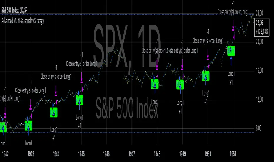
Advanced Multi-Seasonality StrategyThe Multi-Seasonality Strategy is a trading system based on seasonal market patterns. Seasonality refers to recurring market trends driven by predictable calendar-based events. These patterns emerge due to economic cycles, corporate activities (e.g., earnings reports), and investor behavior around specific times of the year. Studies have shown that such effects can influence asset prices over defined periods, leading to opportunities for traders who exploit these patterns (Hirshleifer, 2001; Bouman & Jacobsen, 2002).
How the Strategy Works:
The strategy allows the user to define four distinct periods within a calendar year. For each period, the trader selects:
Entry Date (Month and Day): The date to enter the trade.
Holding Period: The number of trading days to remain in the trade after the entry.
Trade Direction: Whether to take a long or short position during that period.
The system is designed with flexibility, enabling the user to activate or deactivate each of the four periods. The idea is to take advantage of seasonal patterns, such as buying during historically strong periods and selling during weaker ones. A well-known example is the "Sell in May and Go Away" phenomenon, which suggests that stock returns are higher from November to April and weaker from May to October (Bouman & Jacobsen, 2002).
Seasonality in Financial Markets:
Seasonal effects have been documented across different asset classes and markets:
Equities: Stock markets tend to exhibit higher returns during certain months, such as the "January effect," where prices rise after year-end tax-loss selling (Haugen & Lakonishok, 1987).
Commodities: Agricultural commodities often follow seasonal planting and harvesting cycles, which impact supply and demand patterns (Fama & French, 1987).
Forex: Currency pairs may show strength or weakness during specific quarters based on macroeconomic factors, such as fiscal year-end flows or central bank policy decisions.
Scientific Basis:
Research shows that market anomalies like seasonality are linked to behavioral biases and institutional practices. For example, investors may respond to tax incentives at the end of the year, and companies may engage in window dressing (Haugen & Lakonishok, 1987). Additionally, macroeconomic factors, such as monetary policy shifts and holiday trading volumes, can also contribute to predictable seasonal trends (Bouman & Jacobsen, 2002).
Risks of Seasonal Trading:
While the strategy seeks to exploit predictable patterns, there are inherent risks:
Market Changes: Seasonal effects observed in the past may weaken or disappear as market conditions evolve. Increased algorithmic trading, globalization, and policy changes can reduce the reliability of historical patterns (Lo, 2004).
Overfitting: One of the risks in seasonal trading is overfitting the strategy to historical data. A pattern that worked in the past may not necessarily work in the future, especially if it was based on random chance or external factors that no longer apply (Sullivan, Timmermann, & White, 1999).
Liquidity and Volatility: Trading during specific periods may expose the trader to low liquidity, especially around holidays or earnings seasons, leading to slippage and larger-than-expected price swings.
Economic and Geopolitical Shocks: External events such as pandemics, wars, or political instability can disrupt seasonal patterns, leading to unexpected market behavior.
Conclusion:
The Multi-Seasonality Strategy capitalizes on the predictable nature of certain calendar-based patterns in financial markets. By entering and exiting trades based on well-established seasonal effects, traders can potentially capture short-term profits. However, caution is necessary, as market dynamics can change, and seasonal patterns are not guaranteed to persist. Rigorous backtesting, combined with risk management practices, is essential to successfully implementing this strategy.
References:
Bouman, S., & Jacobsen, B. (2002). The Halloween Indicator, "Sell in May and Go Away": Another Puzzle. American Economic Review, 92(5), 1618-1635.
Fama, E. F., & French, K. R. (1987). Commodity Futures Prices: Some Evidence on Forecast Power, Premiums, and the Theory of Storage. Journal of Business, 60(1), 55-73.
Haugen, R. A., & Lakonishok, J. (1987). The Incredible January Effect: The Stock Market's Unsolved Mystery. Dow Jones-Irwin.
Hirshleifer, D. (2001). Investor Psychology and Asset Pricing. Journal of Finance, 56(4), 1533-1597.
Lo, A. W. (2004). The Adaptive Markets Hypothesis: Market Efficiency from an Evolutionary Perspective. Journal of Portfolio Management, 30(5), 15-29.
Sullivan, R., Timmermann, A., & White, H. (1999). Data-Snooping, Technical Trading Rule Performance, and the Bootstrap. Journal of Finance, 54(5), 1647-1691.
This strategy harnesses the power of seasonality but requires careful consideration of the risks and potential changes in market behavior over time.
Statistical ArbitrageThe Statistical Arbitrage Strategy, also known as pairs trading, is a quantitative trading method that capitalizes on price discrepancies between two correlated assets. The strategy assumes that over time, the prices of these two assets will revert to their historical relationship. The core idea is to take advantage of mean reversion, a principle suggesting that asset prices will revert to their long-term average after deviating significantly.
Strategy Mechanics:
1. Selection of Correlated Assets:
• The strategy focuses on two historically correlated assets (e.g., equity index futures like Dow Jones Mini and S&P 500 Mini). These assets tend to move in the same direction due to similar underlying fundamentals, such as overall market conditions. By tracking their relative prices, the strategy seeks to exploit temporary mispricings.
2. Spread Calculation:
• The spread is the difference between the prices of the two assets. This spread represents the relationship between the assets and serves as the basis for determining when to enter or exit trades.
3. Mean and Standard Deviation:
• The historical average (mean) of the spread is calculated using a Simple Moving Average (SMA) over a chosen period. The strategy also computes the standard deviation (volatility) of the spread, which measures how far the spread has deviated from the mean over time. This allows the strategy to define statistically significant price deviations.
4. Entry Signal (Mean Reversion):
• A buy signal is triggered when the spread falls below the mean by a multiple (e.g., two) of the standard deviation. This indicates that one asset is temporarily undervalued relative to the other, and the strategy expects the spread to revert to its mean, generating profits as the prices converge.
5. Exit Signal:
• The strategy exits the trade when the spread reverts to the mean. At this point, the mispricing has been corrected, and the profit from the mean reversion is realized.
Academic Support:
Statistical arbitrage has been widely studied in finance and economics. Gatev, Goetzmann, and Rouwenhorst’s (2006) landmark study on pairs trading demonstrated that this strategy could generate excess returns in equity markets. Their research found that by focusing on historically correlated stocks, traders could identify pricing anomalies and profit from their eventual correction.
Additionally, Avellaneda and Lee (2010) explored statistical arbitrage in different asset classes and found that exploiting deviations in price relationships can offer a robust, market-neutral trading strategy. In these studies, the strategy’s success hinges on the stability of the relationship between the assets and the timely execution of trades when deviations occur.
Risks of Statistical Arbitrage:
1. Correlation Breakdown:
• One of the primary risks is the breakdown of correlation between the two assets. Statistical arbitrage assumes that the historical relationship between the assets will hold in the future. However, market conditions, company fundamentals, or external shocks (e.g., macroeconomic changes) can cause these assets to deviate permanently, leading to potential losses.
• For instance, if two equity indices historically move together but experience divergent economic conditions or policy changes, their prices may no longer revert to the expected mean.
2. Execution Risk:
• This strategy relies on efficient execution and tight spreads. In volatile or illiquid markets, the actual price at which trades are executed may differ significantly from expected prices, leading to slippage and reduced profits.
3. Market Risk:
• Although statistical arbitrage is designed to be market-neutral (i.e., not dependent on the overall market direction), it is not entirely risk-free. Systematic market shocks, such as financial crises or sudden shifts in market sentiment, can affect both assets simultaneously, causing the spread to widen rather than revert to the mean.
4. Model Risk:
• The assumptions underlying the strategy, particularly regarding mean reversion, may not always hold true. The model assumes that asset prices will return to their historical averages within a certain timeframe, but the timing and magnitude of mean reversion can be uncertain. Misestimating this timeframe can lead to extended drawdowns or unrealized losses.
5. Overfitting:
• Over-reliance on historical data to fine-tune the strategy parameters (e.g., the lookback period or standard deviation thresholds) may result in overfitting. This means that the strategy works well on past data but fails to perform in live markets due to changing conditions.
Conclusion:
The Statistical Arbitrage Strategy offers a systematic and quantitative approach to trading that capitalizes on temporary price inefficiencies between correlated assets. It has been proven to generate returns in academic studies and is widely used by hedge funds and institutional traders for its market-neutral characteristics. However, traders must be aware of the inherent risks, including correlation breakdown, execution risks, and the potential for prolonged deviations from the mean. Effective risk management, diversification, and constant monitoring are essential for successfully implementing this strategy in live markets.

Stochastic RSI OHLC StrategyThe script titled "Stochastic RSI High Low Close Bars" is a versatile trading strategy implemented in Pine Script, designed for TradingView. Here's an overview of its features:
Description
This strategy leverages the Stochastic RSI to determine entry and exit signals in the market, focusing on high, low, and close values of the indicator. It incorporates various trading styles, stop-loss mechanisms, and multi-timeframe analysis to adapt to different market conditions.
Key Features
Stochastic RSI Analysis:
Uses the Stochastic RSI to identify potential entry points for long and short positions.
Tracks high, low, and close values for more granular analysis.
Multiple Trading Styles:
Supports diverse trading styles like Volume Color Swing, RSI Divergence, RSI Pullback, and more.
Allows switching between these styles to suit market dynamics.
Session-Based Trading:
Offers session control, limiting trades to specific hours (e.g., NY sessions).
Can close all positions at the end of the trading day.
Stop-Loss and Take-Profit Mechanisms:
Includes both static and dynamic stop-losses, with options for time-based stops, trailing stops, and momentum-based exits.
Customizable take-profit levels ensure efficient trade management.
Volume Analysis:
Integrates volume indicators to add a bias for trade entries and exits, enhancing signal reliability.
Multi-Timeframe Integration:
Employs multi-timeframe RSI analysis, allowing the strategy to capture broader trends and optimize entries.
This script is designed to provide flexibility and adaptability, making it useful for different trading strategies and market conditions. It is suitable for traders looking to refine their entries and exits with a focus on the Stochastic RSI.
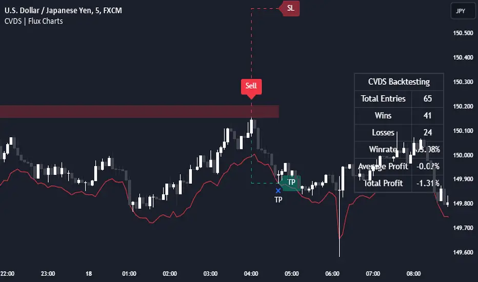
Cumulative Volume Delta Strategy | Flux Charts💎 GENERAL OVERVIEW
Introducing the Cumulative Volume Delta Strategy (CVDS) Indicator, an advanced tool designed to enhance trading strategies by identifying potential trend reversals through volume dynamics. This script features integrated order block detection, Fair Value Gaps (FVGs), and a dynamic take-profit (TP) and stop-loss (SL) system. For an in-depth understanding of the strategy, refer to the "HOW DOES IT WORK?" section below.
Features of the new Cumulative Volume Delta Strategy (CVDS) Indicator :
Cumulative Volume Delta-based Strategy
Order Block and Fair Value Gap (FVG) Entry Methods
Dynamic TP/SL System
Customizable Risk Management Settings
Alerts for Buy, Sell, TP, and SL Signals
📌 HOW DOES IT WORK ?
The CVDS indicator operates by tracking the net volume difference between buyers and sellers to identify divergences that could indicate potential trend reversals. A cumulative volume delta (CVD) calculation is employed to measure the intensity of these divergences in relation to price movements. The net volume sum is reset every trading day (can be changed from the settings using the anchor period option), and divergences are detected when the cumulative volume crosses the 0-line over or under.
Once a significant divergence is detected, the indicator identifies breakout points, confirmed by either Fair Value Gaps (FVGs) or Order Blocks (OBs). Depending on your chosen entry mode, the indicator will trigger a buy or sell entry when the confirmation signal aligns with the breakout direction. Alerts for Buy, Sell, Take-Profit, and Stop-Loss are available.
Note that the indicator cannot run on 1-minute and 1-second charts, as it needs to get data from a lower timeframe. 1-minutes & 1-second timeframes are the minimum timeframes in their ranges respectively.
🚩 UNIQUENESS
What sets this indicator apart is the combination of volume divergence analysis with advanced price action tools like Fair Value Gaps (FVGs) and Order Blocks (OBs). The ability to choose between these methods, along with a dynamic TP/SL system that adapts based on volatility, provides flexibility for traders in any market condition. The backtesting dashboard provides metrics about the performance of the indicator. You can use it to tune the settings for best use in the current ticker. The CVD-based strategy ensures that trades are initiated only when meaningful divergences between volume and price occur, filtering out noise and increasing the likelihood of profitable trades.
⚙️ SETTINGS
1. General Configuration
Anchor Period: Time anchor period used in CVD calculation. This is essentially the period that the volume delta sum will be reset. Lower timeframes may result in more entries at the cost of less reliable results.
Entry Mode: Choose between FVGs or OBs to trigger your entries based on the confirmation signals.
Retracement Requirement: Enable to confirm the entry after a retracement toward the FVG or OB.
2. Fair Value Gaps
FVG Sensitivity: Modify the sensitivity of FVG detection, allowing for more or fewer gaps to be considered valid.
3. Order Blocks (OB)
Swing Length: Define the swing length to identify OB formations. Shorter lengths find smaller OBs, while longer lengths detect larger structures.
4. TP / SL
TP / SL Method:
a) Dynamic: The TP / SL zones will be auto-determined by the algorithm based on the Average True Range (ATR) of the current ticker.
b) Fixed : You can adjust the exact TP / SL ratios from the settings below.
Dynamic Risk: The risk you're willing to take if "Dynamic" TP / SL Method is selected. Higher risk usually means a better winrate at the cost of losing more if the strategy fails. This setting is has a crucial effect on the performance of the indicator, as different tickers may have different volatility so the indicator may have increased performance when this setting is correctly adjusted.
Chande Momentum Oscillator StrategyThe Chande Momentum Oscillator (CMO) Trading Strategy is based on the momentum oscillator developed by Tushar Chande in 1994. The CMO measures the momentum of a security by calculating the difference between the sum of recent gains and losses over a defined period. The indicator offers a means to identify overbought and oversold conditions, making it suitable for developing mean-reversion trading strategies (Chande, 1997).
Strategy Overview:
Calculation of the Chande Momentum Oscillator (CMO):
The CMO formula considers both positive and negative price changes over a defined period (commonly set to 9 days) and computes the net momentum as a percentage.
The formula is as follows:
CMO=100×(Sum of Gains−Sum of Losses)(Sum of Gains+Sum of Losses)
CMO=100×(Sum of Gains+Sum of Losses)(Sum of Gains−Sum of Losses)
This approach distinguishes the CMO from other oscillators like the RSI by using both price gains and losses in the numerator, providing a more symmetrical measurement of momentum (Chande, 1997).
Entry Condition:
The strategy opens a long position when the CMO value falls below -50, signaling an oversold condition where the price may revert to the mean. Research in mean-reversion, such as by Poterba and Summers (1988), supports this approach, highlighting that prices often revert after sharp movements due to overreaction in the markets.
Exit Conditions:
The strategy closes the long position when:
The CMO rises above 50, indicating that the price may have become overbought and may not provide further upside potential.
Alternatively, the position is closed 5 days after the buy signal is triggered, regardless of the CMO value, to ensure a timely exit even if the momentum signal does not reach the predefined level.
This exit strategy aligns with the concept of time-based exits, reducing the risk of prolonged exposure to adverse price movements (Fama, 1970).
Scientific Basis and Rationale:
Momentum and Mean-Reversion:
The strategy leverages the well-known phenomenon of mean-reversion in financial markets. According to research by Jegadeesh and Titman (1993), prices tend to revert to their mean over short periods following strong movements, creating opportunities for traders to profit from temporary deviations.
The CMO captures this mean-reversion behavior by monitoring extreme price conditions. When the CMO reaches oversold levels (below -50), it signals potential buying opportunities, whereas crossing overbought levels (above 50) indicates conditions for selling.
Market Efficiency and Overreaction:
The strategy takes advantage of behavioral inefficiencies and overreactions, which are often the drivers behind sharp price movements (Shiller, 2003). By identifying these extreme conditions with the CMO, the strategy aims to capitalize on the market’s tendency to correct itself when price deviations become too large.
Optimization and Parameter Selection:
The 9-day period used for the CMO calculation is a widely accepted timeframe that balances responsiveness and noise reduction, making it suitable for capturing short-term price fluctuations. Studies in technical analysis suggest that oscillators optimized over such periods are effective in detecting reversals (Murphy, 1999).
Performance and Backtesting:
The strategy's effectiveness is confirmed through backtesting, which shows that using the CMO as a mean-reversion tool yields profitable opportunities. The use of time-based exits alongside momentum-based signals enhances the reliability of the strategy by ensuring that trades are closed even when the momentum signal alone does not materialize.
Conclusion:
The Chande Momentum Oscillator Trading Strategy combines the principles of momentum measurement and mean-reversion to identify and capitalize on short-term price fluctuations. By using a widely tested oscillator like the CMO and integrating a systematic exit approach, the strategy effectively addresses both entry and exit conditions, providing a robust method for trading in diverse market environments.
References:
Chande, T. S. (1997). The New Technical Trader: Boost Your Profit by Plugging into the Latest Indicators. John Wiley & Sons.
Fama, E. F. (1970). Efficient Capital Markets: A Review of Theory and Empirical Work. The Journal of Finance, 25(2), 383-417.
Jegadeesh, N., & Titman, S. (1993). Returns to Buying Winners and Selling Losers: Implications for Stock Market Efficiency. The Journal of Finance, 48(1), 65-91.
Murphy, J. J. (1999). Technical Analysis of the Financial Markets: A Comprehensive Guide to Trading Methods and Applications. New York Institute of Finance.
Poterba, J. M., & Summers, L. H. (1988). Mean Reversion in Stock Prices: Evidence and Implications. Journal of Financial Economics, 22(1), 27-59.
Shiller, R. J. (2003). From Efficient Markets Theory to Behavioral Finance. Journal of Economic Perspectives, 17(1), 83-104.

E9 Bollinger RangeThe E9 Bollinger Range is a technical trading tool that leverages Bollinger Bands to track volatility and price deviations, along with additional trend filtering via EMAs.
The script visually enhances price action with a combination of trend-filtering EMAs, bar colouring for trend direction, signals to indicate potential buy and sell points based on price extension and engulfing patterns.
Here’s a breakdown of its key components:
Bollinger Bands: The strategy plots multiple Bollinger Band deviations to create different price levels. The furthest deviation bands act as warning signs for traders when price extends significantly, signaling potential overbought or oversold conditions.
Bar Colouring: Visual bar colouring is applied to clearly indicate trend direction: green bars for an uptrend and red bars for a downtrend.
EMA Filtering: Two EMAs (50 and 200) are used to help filter out false signals, giving traders a better sense of the underlying trend.
This combination of signals, visual elements, and trend filtering provides traders with a systematic approach to identifying price deviations and taking advantage of market corrections.
Brief History of Bollinger Bands
Bollinger Bands were developed by John Bollinger in the early 1980s as a tool to measure price volatility in financial markets. The bands consist of a moving average (typically 20 periods) with upper and lower bands placed two standard deviations away. These bands expand and contract based on market volatility, offering traders a visual representation of price extremes and potential reversal zones.
John Bollinger’s work revolutionized technical analysis by incorporating volatility into trend detection. His bands remain widely used across markets, including stocks, commodities, and cryptocurrencies. With the ability to highlight overbought and oversold conditions, Bollinger Bands have become a staple in many trading strategies.

Candle Range Theory | Flux Charts💎 GENERAL OVERVIEW
Introducing our new Candle Range Theory Indicator! This powerful tool offers a strategy built around the Candle Range Theory, which analyzes market movements through the relative size and structure of price candles. For more information about the process, check the "HOW DOES IT WORK" section.
Features of the new Candle Range Theory Indicator :
Implementation of the Candle Range Theory
FVG & Order Block Entry Methods
2 Different TP / SL Methods
Customizable Execution Settings
Customizable Backtesting Dashboard
Alerts for Buy, Sell, TP & SL Signals
📌 HOW DOES IT WORK ?
The Candle Range Theory (CRT) indicator operates by identifying significant price movements through the relative size and structure of candlesticks. A key part of the strategy is determining large candles based on their range compared to the Average True Range (ATR) in a higher timeframe. Once identified, a breakout of either the high wick or the low wick of the large candle is required. This breakout is considered a liquidity grab. After that, the indicator waits for confirmation through Fair Value Gaps (FVGs) or Order Blocks (OBs). The confirmation structure must be the opposite direction of the breakout, for example if the high wick is broken, a bearish FVG is required for the short entry. After a confirmation signal is received, the indicator will trigger entry points based on your chosen entry method (FVG or OB), and exit points will be calculated using either a dynamic ATR-based TP/SL method or fixed percentages. Alerts for Buy, Sell, Take-Proft, and Stop-Loss are available.
🚩 UNIQUENESS
This indicator stands out because it combines two highly effective entry methods: Fair Value Gaps (FVGs) and Order Blocks (OBs). You can choose between these strategies depending on market conditions. Additionally, the dynamic TP/SL system uses the ticker's volatility to automatically calculate stop-loss and take-profit targets. The backtesting dashboard provides metrics about the performance of the indicator. You can use it to tune the settings for best use in the current tiker. The Candle Range Theory approach offers more flexibility compared to traditional indicators, allowing for better customization and control based on your risk tolerance.
⚙️ SETTINGS
1. General Configuration
Higher Timeframe: Customize the higher timeframe for analysis. Recommended combinations include M15 -> H4, H4 -> Daily, Daily -> Weekly, and Weekly -> Monthly.
HTF Candle Size: Define the size of the higher timeframe candles as Big, Normal, or Small to filter valid setups based on their range relative to ATR.
Entry Mode: Choose between FVGs and Order Blocks for your entry triggers.
Require Retracement: Enable this option if you want a retracement to the FVG or OB for entry confirmation.
Show HTF Candle Lines: Toggle to display the higher timeframe candle lines for better visual clarity.
2. Fair Value Gaps
FVG Sensitivity: You may select between Low, Normal, High or Extreme FVG detection sensitivity. This will essentially determine the size of the spotted FVGs, with lower sensitivities resulting in spotting bigger FVGs, and higher sensitivities resulting in spotting all sizes of FVGs.
3. Order Blocks
Swing Length: Swing length is used when finding order block formations. Smaller values will result in finding smaller order blocks.
4. TP / SL
TP / SL Method:
a) Dynamic: The TP / SL zones will be auto-determined by the algorithm based on the Average True Range (ATR) of the current ticker.
b) Fixed : You can adjust the exact TP / SL ratios from the settings below.
Dynamic Risk: The risk you're willing to take if "Dynamic" TP / SL Method is selected. Higher risk usually means a better winrate at the cost of losing more if the strategy fails. This setting is has a crucial effect on the performance of the indicator, as different tickers may have different volatility so the indicator may have increased performance when this setting is correctly adjusted.

Futures Beta Overview with Different BenchmarksBeta Trading and Its Implementation with Futures
Understanding Beta
Beta is a measure of a security's volatility in relation to the overall market. It represents the sensitivity of the asset's returns to movements in the market, typically benchmarked against an index like the S&P 500. A beta of 1 indicates that the asset moves in line with the market, while a beta greater than 1 suggests higher volatility and potential risk, and a beta less than 1 indicates lower volatility.
The Beta Trading Strategy
Beta trading involves creating positions that exploit the discrepancies between the theoretical (or expected) beta of an asset and its actual market performance. The strategy often includes:
Long Positions on High Beta Assets: Investors might take long positions in assets with high beta when they expect market conditions to improve, as these assets have the potential to generate higher returns.
Short Positions on Low Beta Assets: Conversely, shorting low beta assets can be a strategy when the market is expected to decline, as these assets tend to perform better in down markets compared to high beta assets.
Betting Against (Bad) Beta
The paper "Betting Against Beta" by Frazzini and Pedersen (2014) provides insights into a trading strategy that involves betting against high beta stocks in favor of low beta stocks. The authors argue that high beta stocks do not provide the expected return premium over time, and that low beta stocks can yield higher risk-adjusted returns.
Key Points from the Paper:
Risk Premium: The authors assert that investors irrationally demand a higher risk premium for holding high beta stocks, leading to an overpricing of these assets. Conversely, low beta stocks are often undervalued.
Empirical Evidence: The paper presents empirical evidence showing that portfolios of low beta stocks outperform portfolios of high beta stocks over long periods. The performance difference is attributed to the irrational behavior of investors who overvalue riskier assets.
Market Conditions: The paper suggests that the underperformance of high beta stocks is particularly pronounced during market downturns, making low beta stocks a more attractive investment during volatile periods.
Implementation of the Strategy with Futures
Futures contracts can be used to implement the betting against beta strategy due to their ability to provide leveraged exposure to various asset classes. Here’s how the strategy can be executed using futures:
Identify High and Low Beta Futures: The first step involves identifying futures contracts that have high beta characteristics (more sensitive to market movements) and those with low beta characteristics (less sensitive). For example, commodity futures like crude oil or agricultural products might exhibit high beta due to their price volatility, while Treasury bond futures might show lower beta.
Construct a Portfolio: Investors can construct a portfolio that goes long on low beta futures and short on high beta futures. This can involve trading contracts on stock indices for high beta stocks and bonds for low beta exposures.
Leverage and Risk Management: Futures allow for leverage, which means that a small movement in the underlying asset can lead to significant gains or losses. Proper risk management is essential, using stop-loss orders and position sizing to mitigate the inherent risks associated with leveraged trading.
Adjusting Positions: The positions may need to be adjusted based on market conditions and the ongoing performance of the futures contracts. Continuous monitoring and rebalancing of the portfolio are essential to maintain the desired risk profile.
Performance Evaluation: Finally, investors should regularly evaluate the performance of the portfolio to ensure it aligns with the expected outcomes of the betting against beta strategy. Metrics like the Sharpe ratio can be used to assess the risk-adjusted returns of the portfolio.
Conclusion
Beta trading, particularly the strategy of betting against high beta assets, presents a compelling approach to capitalizing on market inefficiencies. The research by Frazzini and Pedersen emphasizes the benefits of focusing on low beta assets, which can yield more favorable risk-adjusted returns over time. When implemented using futures, this strategy can provide a flexible and efficient means to execute trades while managing risks effectively.
References
Frazzini, A., & Pedersen, L. H. (2014). Betting against beta. Journal of Financial Economics, 111(1), 1-25.
Fama, E. F., & French, K. R. (1992). The cross-section of expected stock returns. Journal of Finance, 47(2), 427-465.
Black, F. (1972). Capital Market Equilibrium with Restricted Borrowing. Journal of Business, 45(3), 444-454.
Ang, A., & Chen, J. (2010). Asymmetric volatility: Evidence from the stock and bond markets. Journal of Financial Economics, 99(1), 60-80.
By utilizing the insights from academic literature and implementing a disciplined trading strategy, investors can effectively navigate the complexities of beta trading in the futures market.

Overnight Positioning w EMA - Strategy [presentTrading]I've recently started researching Market Timing strategies, and it’s proving to be quite an interesting area of study. The idea of predicting optimal times to enter and exit the market, based on historical data and various indicators, brings a dynamic edge to trading. Additionally, it is integrated with the 3commas bot for automated trade execution.
I'm still working on it. Welcome to share your point of view.
█ Introduction and How it is Different
The "Overnight Positioning with EMA " is designed to capitalize on market inefficiencies during the overnight trading period. This strategy takes a position shortly before the market closes and exits shortly after it opens the following day. What sets this strategy apart is the integration of an optional Exponential Moving Average (EMA) filter, which ensures that trades are aligned with the underlying trend. The strategy provides flexibility by allowing users to select between different global market sessions, such as the US, Asia, and Europe.
It is integrated with the 3commas bot for automated trade execution and has a built-in mechanism to avoid holding positions over the weekend by force-closing positions on Fridays before the market closes.
BTCUSD 20 mins Performance
█ Strategy, How it Works: Detailed Explanation
The core logic of this strategy is simple: enter trades before market close and exit them after market open, taking advantage of potential price movements during the overnight period. Here’s how it works in more detail:
🔶 Market Timing
The strategy determines the local market open and close times based on the selected market (US, Asia, Europe) and adjusts entry and exit points accordingly. The entry is triggered a specific number of minutes before market close, and the exit is triggered a specific number of minutes after market open.
🔶 EMA Filter
The strategy includes an optional EMA filter to help ensure that trades are taken in the direction of the prevailing trend. The EMA is calculated over a user-defined timeframe and length. The entry is only allowed if the closing price is above the EMA (for long positions), which helps to filter out trades that might go against the trend.
The EMA formula:
```
EMA(t) = +
```
Where:
- EMA(t) is the current EMA value
- Close(t) is the current closing price
- n is the length of the EMA
- EMA(t-1) is the previous period's EMA value
🔶 Entry Logic
The strategy monitors the market time in the selected timezone. Once the current time reaches the defined entry period (e.g., 20 minutes before market close), and the EMA condition is satisfied, a long position is entered.
- Entry time calculation:
```
entryTime = marketCloseTime - entryMinutesBeforeClose * 60 * 1000
```
🔶 Exit Logic
Exits are triggered based on a specified time after the market opens. The strategy checks if the current time is within the defined exit period (e.g., 20 minutes after market open) and closes any open long positions.
- Exit time calculation:
exitTime = marketOpenTime + exitMinutesAfterOpen * 60 * 1000
🔶 Force Close on Fridays
To avoid the risk of holding positions over the weekend, the strategy force-closes any open positions 5 minutes before the market close on Fridays.
- Force close logic:
isFriday = (dayofweek(currentTime, marketTimezone) == dayofweek.friday)
█ Trade Direction
This strategy is designed exclusively for long trades. It enters a long position before market close and exits the position after market open. There is no shorting involved in this strategy, and it focuses on capturing upward momentum during the overnight session.
█ Usage
This strategy is suitable for traders who want to take advantage of price movements that occur during the overnight period without holding positions for extended periods. It automates entry and exit times, ensuring that trades are placed at the appropriate times based on the market session selected by the user. The 3commas bot integration also allows for automated execution, making it ideal for traders who wish to set it and forget it. The strategy is flexible enough to work across various global markets, depending on the trader's preference.
█ Default Settings
1. entryMinutesBeforeClose (Default = 20 minutes):
This setting determines how many minutes before the market close the strategy will enter a long position. A shorter duration could mean missing out on potential movements, while a longer duration could expose the position to greater price fluctuations before the market closes.
2. exitMinutesAfterOpen (Default = 20 minutes):
This setting controls how many minutes after the market opens the position will be exited. A shorter exit time minimizes exposure to market volatility at the open, while a longer exit time could capture more of the overnight price movement.
3. emaLength (Default = 100):
The length of the EMA affects how the strategy filters trades. A shorter EMA (e.g., 50) reacts more quickly to price changes, allowing more frequent entries, while a longer EMA (e.g., 200) smooths out price action and only allows entries when there is a stronger underlying trend.
The effect of using a longer EMA (e.g., 200) would be:
```
EMA(t) = +
```
4. emaTimeframe (Default = 240):
This is the timeframe used for calculating the EMA. A higher timeframe (e.g., 360) would base entries on longer-term trends, while a shorter timeframe (e.g., 60) would respond more quickly to price movements, potentially allowing more frequent trades.
5. useEMA (Default = true):
This toggle enables or disables the EMA filter. When enabled, trades are only taken when the price is above the EMA. Disabling the EMA allows the strategy to enter trades without any trend validation, which could increase the number of trades but also increase risk.
6. Market Selection (Default = US):
This setting determines which global market's open and close times the strategy will use. The selection of the market affects the timing of entries and exits and should be chosen based on the user's preference or geographic focus.

Martingale with MACD+KDJ opening conditionsStrategy Overview:
This strategy is based on a Martingale trading approach, incorporating MACD and KDJ indicators. It features pyramiding, trailing stops, and dynamic profit-taking mechanisms, suitable for both long and short trades. The strategy increases position size progressively using a Multiplier, a key feature of Martingale systems.
Key Concepts:
Martingale Strategy: A trading system where positions are doubled or increased after a loss to recover previous losses with a single successful trade. In this script, the position size is incremented using a Multiplier for each addition.
Pyramiding: Allows adding to existing trades when market conditions are favorable, enhancing profitability during trends.
Settings:
Basic Inputs:
Initial Order: Defines the starting size of the position.
Default: 150.0
MACD Settings: Customize the fast, slow, and signal smoothing lengths.
Default: Fast Length: 9, Slow Length: 26, Signal Smoothing: 9
KDJ Settings: Customize the length and smoothing parameters for KDJ.
Default: Length: 14, Smooth K: 3, Smooth D: 3
Max Additions: Sets the number of additional positions (pyramiding).
Default: 5 (Min: 1, Max: 10)
Position Sizing: Percent to add to positions on favorable conditions.
Default: 1.0%
Martingale Multiplier:
Add Multiplier: This value controls the scaling of additional positions according to the Martingale principle. After each loss, a new position is added, and its size is increased by the Multiplier factor. For example, with a multiplier of 2, each new addition will be twice as large as the previous one, accelerating recovery if the price moves favorably.
Default: 1.0 (no multiplication)
Can be adjusted up to 10x to aggressively increase position size after losses.
Trade Execution:
Long Trades:
Entry Condition: A long position is opened when the MACD line crosses over the signal line, and the KDJ’s %K crosses above %D.
Additions (Martingale): After the initial long position, new positions are added if the price drops by the defined percentage, and each new addition is increased using the Multiplier. This continues up to the set Max Additions.
Short Trades:
Entry Condition: A short position is opened when the MACD line crosses under the signal line, and the KDJ’s %K crosses below %D.
Additions (Martingale): After the initial short position, new positions are added if the price rises by the defined percentage, and each new addition is increased using the Multiplier.
Exit Conditions:
Take Profit: Exits are triggered when the price reaches the take-profit threshold.
Stop Loss: If the price moves unfavorably, the position will be closed at the set stop-loss level.
Trailing Stop: Adjusts dynamically as the price moves in favor of the trade to lock in profits.
On-Chart Visuals:
Long Signals: Blue triangles below the bars indicate long entries, and green triangles mark additional long positions.
Short Signals: Red triangles above the bars indicate short entries, and orange triangles mark additional short positions.
Information Table:
The strategy displays a table with key metrics:
Open Price: The entry price of the trade.
Average Price: The average price of the current position.
Additions: The number of additional positions taken.
Next Add Price: The price level for the next position.
Take Profit: The price at which profits will be taken.
Stop Loss: The stop-loss level to minimize risk.
Usage Instructions:
Adjust the parameters to your trading style using the input settings.
The Multiplier amplifies your position size after each addition, so use it cautiously, especially in volatile markets.
Monitor the signals and table on the chart for entry/exit decisions and trade management.

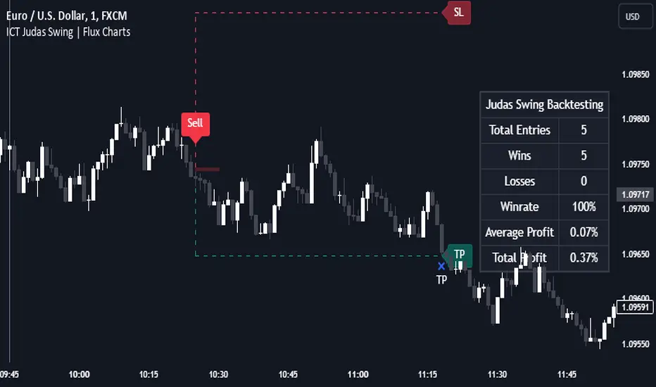
ICT Judas Swing | Flux Charts💎 GENERAL OVERVIEW
Introducing our new ICT Judas Swing Indicator! This indicator is built around the ICT's "Judas Swing" strategy. The strategy looks for a liquidity grab around NY 9:30 session and a Fair Value Gap for entry confirmation. For more information about the process, check the "HOW DOES IT WORK" section.
Features of the new ICT Judas Swing :
Implementation of ICT's Judas Swing Strategy
2 Different TP / SL Methods
Customizable Execution Settings
Customizable Backtesting Dashboard
Alerts for Buy, Sell, TP & SL Signals
📌 HOW DOES IT WORK ?
The strategy begins by identifying the New York session from 9:30 to 9:45 and marking recent liquidity zones. These liquidity zones are determined by locating high and low pivot points: buyside liquidity zones are identified using high pivots that haven't been invalidated, while sellside liquidity zones are found using low pivots. A break of either buyside or sellside liquidity must occur during the 9:30-9:45 session, which is interpreted as a liquidity grab by smart money. The strategy assumes that after this liquidity grab, the price will reverse and move in the opposite direction. For entry confirmation, a fair value gap (FVG) in the opposite direction of the liquidity grab is required. A buyside liquidity grab calls for a bearish FVG, while a sellside grab requires a bullish FVG. Based on the type of FVG—bullish for buys and bearish for sells—the indicator will then generate a Buy or Sell signal.
After the Buy or Sell signal, the indicator immediately draws the take-profit (TP) and stop-loss (SL) targets. The indicator has three different TP & SL modes, explained in the "Settings" section of this write-up.
You can set up alerts for entry and TP & SL signals, and also check the current performance of the indicator and adjust the settings accordingly to the current ticker using the backtesting dashboard.
🚩 UNIQUENESS
This indicator is an all-in-one suit for the ICT's Judas Swing concept. It's capable of plotting the strategy, giving signals, a backtesting dashboard and alerts feature. Different and customizable algorithm modes will help the trader fine-tune the indicator for the asset they are currently trading. Three different TP / SL modes are available to suit your needs. The backtesting dashboard allows you to see how your settings perform in the current ticker. You can also set up alerts to get informed when the strategy is executable for different tickers.
⚙️ SETTINGS
1. General Configuration
Swing Length -> The swing length for pivot detection. Higher settings will result in
FVG Detection Sensitivity -> You may select between Low, Normal, High or Extreme FVG detection sensitivity. This will essentially determine the size of the spotted FVGs, with lower sensitivies resulting in spotting bigger FVGs, and higher sensitivies resulting in spotting all sizes of FVGs.
2. TP / SL
TP / SL Method ->
a) Dynamic: The TP / SL zones will be auto-determined by the algorithm based on the Average True Range (ATR) of the current ticker.
b) Fixed : You can adjust the exact TP / SL ratios from the settings below.
Dynamic Risk -> The risk you're willing to take if "Dynamic" TP / SL Method is selected. Higher risk usually means a better winrate at the cost of losing more if the strategy fails. This setting is has a crucial effect on the performance of the indicator, as different tickers may have different volatility so the indicator may have increased performance when this setting is correctly adjusted.
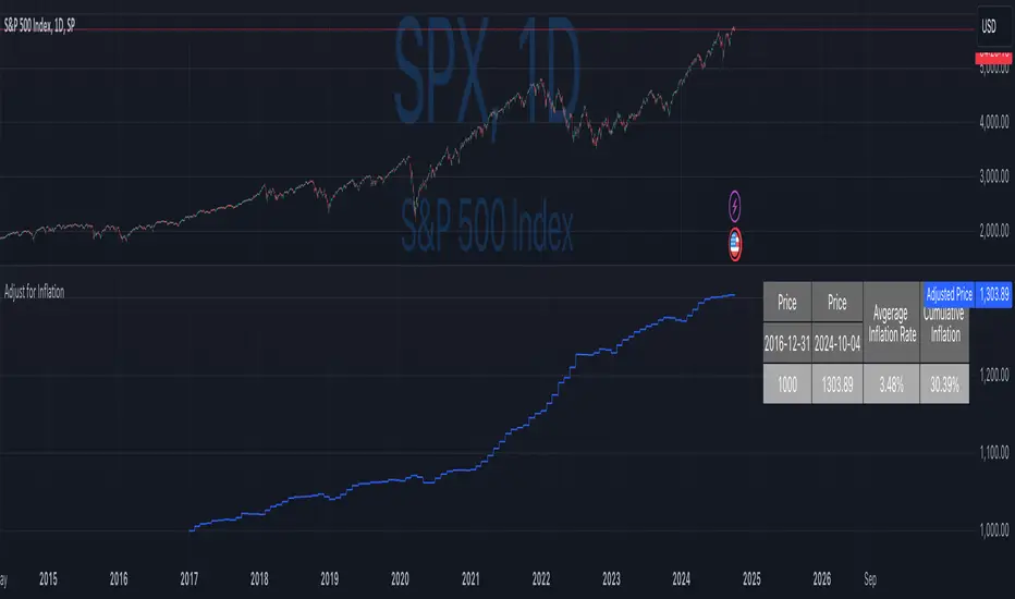
Inflation-Adjusted Price IndicatorThis indicator allows traders to adjust historical prices for inflation using customizable CPI data. The script computes the adjusted price by selecting a reference date, the original price, and the CPI source (US CPI or custom input) and plots it as a line on the chart. Additionally, a table summarizes the adjusted price values and average and total inflation rates.
While the indicator serves as a standalone tool to understand inflation's impact on prices, it is a supportive element in more advanced trading strategies requiring accurate analysis of inflation-adjusted data.
Disclaimer
Please remember that past performance may not be indicative of future results.
Due to various factors, including changing market conditions, the strategy may no longer perform as well as in historical backtesting.
This post and the script don’t provide any financial advice.
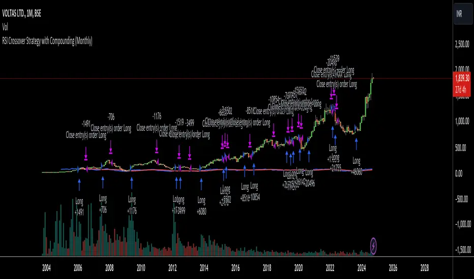
RSI Crossover Strategy with Compounding (Monthly)Explanation of the Code:
Initial Setup:
The strategy initializes with a capital of 100,000.
Variables track the capital and the amount invested in the current trade.
RSI Calculation:
The RSI and its SMA are calculated on the monthly timeframe using request.security().
Entry and Exit Conditions:
Entry: A long position is initiated when the RSI is above its SMA and there’s no existing position. The quantity is based on available capital.
Exit: The position is closed when the RSI falls below its SMA. The capital is updated based on the net profit from the trade.
Capital Management:
After closing a trade, the capital is updated with the net profit plus the initial investment.
Plotting:
The RSI and its SMA are plotted for visualization on the chart.
A label displays the current capital.
Notes:
Test the strategy on different instruments and historical data to see how it performs.
Adjust parameters as needed for your specific trading preferences.
This script is a basic framework, and you might want to enhance it with risk management, stop-loss, or take-profit features as per your trading strategy.
Feel free to modify it further based on your needs!
KAMA Cloud STIndicator:
Description:
The KAMA Cloud indicator is a sophisticated trading tool designed to provide traders with insights into market trends and their intensity. This indicator is built on the Kaufman Adaptive Moving Average (KAMA), which dynamically adjusts its sensitivity to filter out market noise and respond to significant price movements. The KAMA Cloud leverages multiple KAMAs to gauge trend direction and strength, offering a visual representation that is easy to interpret.
How It Works:
The KAMA Cloud uses twenty different KAMA calculations, each set to a distinct lookback period ranging from 5 to 100. These KAMAs are calculated using the average of the open, high, low, and close prices (OHLC4), ensuring a balanced view of price action. The relative positioning of these KAMAs helps determine the direction of the market trend and its momentum.
By measuring the cumulative relative distance between these KAMAs, the indicator effectively assesses the overall trend strength, akin to how the Average True Range (ATR) measures market volatility. This cumulative measure helps in identifying the trend’s robustness and potential sustainability.
The visualization component of the KAMA Cloud is particularly insightful. It plots a 'cloud' formed between the base KAMA (set at a 100-period lookback) and an adjusted KAMA that incorporates the cumulative relative distance scaled up. This cloud changes color based on the trend direction — green for upward trends and red for downward trends, providing a clear, visual representation of market conditions.
How the Strategy Works:
The KAMA Cloud ST strategy employs multiple KAMA calculations with varying lengths to capture the nuances of market trends. It measures the relative distances between these KAMAs to determine the trend's direction and strength, much like the original indicator. The strategy enhances decision-making by plotting a 'cloud' formed between the base KAMA (set to a 100-period lookback) and an adjusted KAMA that scales according to the cumulative relative distance of all KAMAs.
Key Components of the Strategy:
Multiple KAMA Layers: The strategy calculates KAMAs for periods ranging from 5 to 100 to analyze short to long-term market trends.
Dynamic Cloud: The cloud visually represents the trend’s strength and direction, updating in real-time as the market evolves.
Signal Generation: Trade signals are generated based on the orientation of the cloud relative to a smoothed version of the upper KAMA boundary. Long positions are initiated when the market trend is upward, and the current cloud value is above its smoothed average. Conversely, positions are closed when the trend reverses, indicated by the cloud falling below the smoothed average.
Suggested Usage:
Market: Stocks, not cryptocurrency
Timeframe: 1 Hour
Indicator:

Commitment of Trader %R StrategyThis Pine Script strategy utilizes the Commitment of Traders (COT) data to inform trading decisions based on the Williams %R indicator. The script operates in TradingView and includes various functionalities that allow users to customize their trading parameters.
Here’s a breakdown of its key components:
COT Data Import:
The script imports the COT library from TradingView to access historical COT data related to different trader groups (commercial hedgers, large traders, and small traders).
User Inputs:
COT data selection mode (e.g., Auto, Root, Base currency).
Whether to include futures, options, or both.
The trader group to analyze.
The lookback period for calculating the Williams %R.
Upper and lower thresholds for triggering trades.
An option to enable or disable a Simple Moving Average (SMA) filter.
Williams %R Calculation: The script calculates the Williams %R value, which is a momentum indicator that measures overbought or oversold levels based on the highest and lowest prices over a specified period.
SMA Filter: An optional SMA filter allows users to limit trades to conditions where the price is above or below the SMA, depending on the configuration.
Trade Logic: The strategy enters long positions when the Williams %R value exceeds the upper threshold and exits when the value falls below it. Conversely, it enters short positions when the Williams %R value is below the lower threshold and exits when the value rises above it.
Visual Elements: The script visually indicates the Williams %R values and thresholds on the chart, with the option to plot the SMA if enabled.
Commitment of Traders (COT) Data
The COT report is a weekly publication by the Commodity Futures Trading Commission (CFTC) that provides a breakdown of open interest positions held by different types of traders in the U.S. futures markets. It is widely used by traders and analysts to gauge market sentiment and potential price movements.
Data Collection: The COT data is collected from futures commission merchants and is published every Friday, reflecting positions as of the previous Tuesday. The report categorizes traders into three main groups:
Commercial Traders: These are typically hedgers (like producers and processors) who use futures to mitigate risk.
Non-Commercial Traders: Often referred to as speculators, these traders do not have a commercial interest in the underlying commodity but seek to profit from price changes.
Non-reportable Positions: Small traders who do not meet the reporting threshold set by the CFTC.
Interpretation:
Market Sentiment: By analyzing the positions of different trader groups, market participants can gauge sentiment. For instance, if commercial traders are heavily short, it may suggest they expect prices to decline.
Extreme Positions: Some traders look for extreme positions among non-commercial traders as potential reversal signals. For example, if speculators are overwhelmingly long, it might indicate an overbought condition.
Statistical Insights: COT data is often used in conjunction with technical analysis to inform trading decisions. Studies have shown that analyzing COT data can provide valuable insights into future price movements (Lund, 2018; Hurst et al., 2017).
Scientific References
Lund, J. (2018). Understanding the COT Report: An Analysis of Speculative Trading Strategies.
Journal of Derivatives and Hedge Funds, 24(1), 41-52. DOI:10.1057/s41260-018-00107-3
Hurst, B., O'Neill, R., & Roulston, M. (2017). The Impact of COT Reports on Futures Market Prices: An Empirical Analysis. Journal of Futures Markets, 37(8), 763-785.
DOI:10.1002/fut.21849
Commodity Futures Trading Commission (CFTC). (2024). Commitment of Traders. Retrieved from CFTC Official Website.

Big 5 Checklist | XEONEDIAThe Big 5 Checklist | XEONEDIA indicator is a powerful trading tool designed to help traders prepare their trading decisions in a structured and effective manner. The indicator encompasses five key areas:
Strategy Documentation :
✅ Ensure that the trading strategy is clearly defined and documented.
✅ Conduct backtesting.
✅ Perform demo testing with an 80% success rate.
✅ Analyze trading results.
✅ Regularly refine the strategy.
Risk Management :
✅ Minimize financial losses and ensure responsible trading.
✅ Set a risk limit of 1-2%.
✅ Use stop-loss orders.
✅ Ensure a risk-reward ratio of at least 2:1.
✅ Adjust position sizes.
Technical Analysis :
✅ Evaluate charts and indicators to identify trading opportunities.
✅ Identify support and resistance levels.
✅ Use technical indicators (e.g., RSI).
✅ Set entry and exit points.
✅ Establish alerts for specific market conditions.
Market Conditions :
✅ Consider external factors that may influence trading.
✅ Monitor the economic calendar.
✅ Apply fundamental analysis.
✅ Observe market volatility.
✅ Analyze global trends.
Psychological Management :
✅ Control emotions and mindset during trading.
✅ Adhere to the trading plan.
✅ Manage emotions while trading.
✅ Set realistic expectations.
✅ Take regular mental breaks.
Mastercheck
The Mastercheck provides a digital checklist where traders can track their progress live. Users can make their own notes and view their checklist on any TradingView device, ensuring they stay informed about their trading readiness and can make adjustments in real-time. ✅
Overall, the Big 5 Checklist | XEONEDIA indicator helps minimize risks and maximize the chances of successful trades by promoting systematic and comprehensive trading preparation.